PlotProcessor examples
Putting together the features offered by the PlotProcessor allows the creation of plots for a very diverse range of use-cases. Below are a few examples of PlotProcessor outputs together with the full configurations used to generated them.
Example 1: two histograms and difference
A common use for the bottom pad is to show the relation between objects
drawn in the top pad, such as ratios or differences. The example below
demonstrates how to create a two-pad layout using the pads
key in the figure configuration and assign plots to pads using the
pad key in the plot configuration, as well as a few other
features described above.
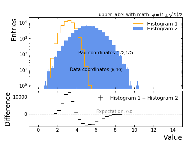
Example plot demonstrating a two-pad layout
from Karma.PostProcessing.Palisade import PlotProcessor, LiteralString

cfg = {
  # declare input files
  'input_files' : {
    'my_file' : "input_file.root"
  },

  # declare figures (only one in this example)
  'figures' : [

    # define the figure
    {
      # output file name (extension determines file type)
      'filename': 'demonstration_plot.png',

      # list of plots (one dict per plot)
      'subplots': [

        # plot histograms from 'my_file'
        {
          'expression' : '"my_file:h1"',
          'plot_method': 'step',
          'color': 'orange',
          'label': "Histogram 1",
          'pad': 0,
        },
        {
          'expression' : '"my_file:h2"',
          'plot_method': 'bar',
          'color': 'cornflowerblue',
          'label': "Histogram 2",
          'pad': 0,
        },
        # plot difference of above histograms in bottom pad
        {
          'expression' : '"my_file:h1" - "my_file:h2"',
          'plot_method': 'errorbar',
          'label': "Histogram 1 $-$ Histogram 2",
          'color': 'black',
          'pad': 1,
        }
      ],

      # adjust layout
      'pad_spec': {
        # set margins
        'left': 0.15,
        'right': 0.95,
        'bottom': 0.12,
        # set vertical pad spacing
        'hspace': 0.04,
      },

      # define pads (a main pad and a pad for the difference)
      'pads': [
        # pad 0
        {
          'height_share': 2,  # make pad two units high
          'y_label' : 'Entries',
          'y_scale' : 'log',  # use logarithmic scaling for 'y' axis

          'x_range' : (-1, 15),
          'x_ticklabels': [],  # do not display tick labels for upper pad
        },
        # pad 1
        {
          'height_share': 1,  # make pad one unit high
          'y_label' : 'Difference',

          'x_label' : 'Value',
          'x_range' : (-1, 15),  # set x range to match the pad above

          'axhlines' : [0.0],  # draw a reference line at zero
        }
      ],

      'texts' : [
        {
          'text': 'Pad coordinates $(1/2, 1/2)$',
          'xy': (.5, .5),
          'xycoords': 'axes fraction',  # default: 'xy' are fraction of pad dimensions
          # matplotlib keywords
          'ha': 'center',  # align text horizontally
          'va': 'center'   # align text vertically
        },
        {
          'text': 'Data coordinates $(6, 10)$',
          'xy': (6, 10),
          'xycoords': 'data',  # 'xy' are data coordinates
          # matplotlib keywords
          'ha': 'center',
          'va': 'center'
        },
        {
          'text': 'Expectation: $0.0$',
          'xy': (6, 500),
          'xycoords': 'data',
          'pad': 1,  # put this text in lower pad
          # matplotlib keywords
          'color': 'gray'
        },
        # upper plot label (need to escape braces with `LiteralString`)
        {
          'text' : LiteralString(r"upper label with math: $\phi={\left(1\pm\sqrt{5}\right)}/{2}$"),
          'xy': (1, 1),
          'xycoords': 'axes fraction',
          'xytext': (0, 5),
          'textcoords': 'offset points',
          'pad': 0
        }
      ],
    }
  ],

  'expansions' : {}  # not needed, but left in for completeness
}

p = PlotProcessor(cfg, output_folder='.')
p.run()
Example 2: stacked histograms and fraction of total
Histograms with the same binning can be stacked on top of each other by
providing a stack keyword in the corresponding subplot
configuration. All subplots that are plotted in the same pad and have
the same stack will be stacked.
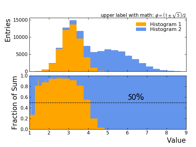
Example plot deomnstrating stacking
from Karma.PostProcessing.Palisade import PlotProcessor, LiteralString

cfg = {
  # declare input files
  'input_files' : {
    'my_file' : "input_file.root"
  },

  # declare figures (only one in this example)
  'figures' : [

    # define the figure
    {
          # output file name (extension determines file type)
      'filename': 'demonstration_plot_2.png',

      # list of plots (one dict per plot)
      'subplots': [

        # plot histograms from 'my_file'
        {
          'expression' : '"my_file:h1"',
          'plot_method': 'bar',
          'color': 'orange',
          'label': "Histogram 1",
          'stack': 'my_stack',  # give the stack a name
          'pad': 0,
        },
        {
          'expression' : '"my_file:h2"',
          'plot_method': 'bar',
          'color': 'cornflowerblue',
          'label': "Histogram 2",
          'stack': 'my_stack',
          'pad': 0,
        },
        # plot fractions to total
        {
          'expression' : '"my_file:h1" / ("my_file:h1" + "my_file:h2")',
          'plot_method': 'bar',
          #'label': "Histogram 2",  # no legend entry in bottom pad
          'color': 'orange',
          'stack': 'my_stack',  # new stack in bottom pad despite identical name
          'pad': 1,
        },
        {
          'expression' : '"my_file:h2" / ("my_file:h1" + "my_file:h2")',
          'plot_method': 'bar',
          #'label': "Histogram 2",  # no legend entry in bottom pad
          'color': 'cornflowerblue',
          'stack': 'my_stack',
          'pad': 1,
        }
      ],

      # adjust layout
      'pad_spec': {
        # set margins
        'left': 0.15,
        'right': 0.95,
        'bottom': 0.12,
        # set vertical pad spacing
        'hspace': 0.08,
      },

      # define pads (a main pad and a pad for the fractions)
      'pads': [
        # pad 0
        {
          'height_share': 1,  # make pad one unit high
          'y_label' : 'Entries',
          'y_scale' : 'linear',
          'x_range' : (1, 9),
          'x_ticklabels': [],  # do not display tick labels for upper pad
        },
        # pad 1
        {
          'height_share': 1,  # make pad one unit high
          'y_label' : 'Fraction of Sum',
          'y_range' : (0, 1),
          'x_label' : 'Value',
          'x_range' : (1, 9),
          # high 'zorder' needed, line otherwise hidden by bars
          'axhlines' : [dict(values=[0.5], color='black', zorder=100)],
        }
      ],

      'texts' : [
          {
            'text': "$50$%",
            'xy': (6, 0.55),
            'xycoords': 'data',
            'fontsize': 20,
            'pad': 1,
          },
          # upper plot label (need to escape braces with `LiteralString`)
          {
            'text' : LiteralString(r"upper label with math: $\phi={\left(1\pm\sqrt{5}\right)}/{2}$"),
            'xy': (1, 1),
            'xycoords': 'axes fraction',
            'xytext': (0, 5),
            'textcoords': 'offset points',
            'pad': 0
          }
      ],

    }
  ],

  'expansions' : {}  # not needed, but left in for completeness
}

p = PlotProcessor(cfg, output_folder='.')
p.run()
Example 3: plot of 2D histogram using a colormap
Two-dimensional histograms can be plotted by representing the bins as colored patches in the x–y plane. The bin value will be mapped to a continuous sequence of colors called a colormap.
The matplotlib library supports plotting two-dimensional histograms
via the plot method pcolormesh. The colormap can be set
via the cmap keyword.
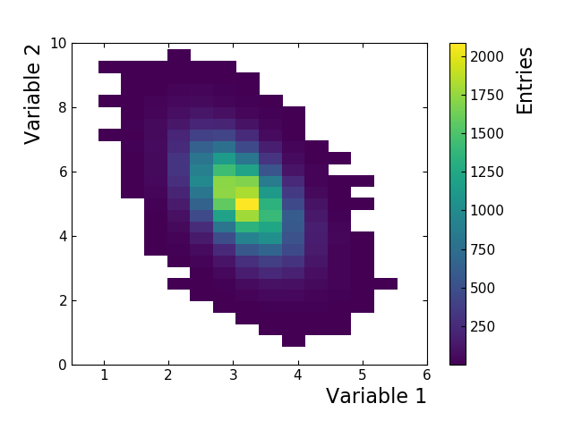
Two-dimensional histogram plotted using pcolormesh.
from Karma.PostProcessing.Palisade import PlotProcessor, LiteralString

cfg = {
  # declare input files
  'input_files' : {
    'my_file' : "input_file.root"
  },

  # declare figures (only one in this example)
  'figures' : [

    # define the figure
    {
      # output file name (extension determines file type)
      'filename': 'demonstration_plot_3.png',

      # list of plots (one dict per plot)
      'subplots': [

        # plot object 'h2d' from 'my_file'
        {
          'expression' : '"my_file:h2d"',
          'plot_method' : 'pcolormesh',
          'cmap' : 'viridis',
        }
      ],

      # adjust layout
      'pad_spec': {
        # set margins
        'top': 0.90,
        'bottom': 0.15,
      },

      # define pads (only one pad)
      'pads': [
        {
          'x_label': 'Variable 1',
          'y_label': 'Variable 2',
          'x_range': (0.5, 6.0),
          'y_range': (0, 10),
          'z_label': 'Entries',  # colorbar label
          # add space between colorbar and its label
          'z_labelpad': 25,
        }
      ]
    }
  ],

  'expansions' : {}
}

p = PlotProcessor(cfg, output_folder='.')
p.run()
Todo
Add more examples.